First Play With PCA
Click
on the “Data set” button
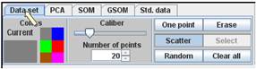
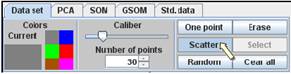
Use
the “Scatter” button with various “Caliber” and “Number of points” values; in
addition, you may add several random points using the button “Random”.
Prepare
the cloud of data points
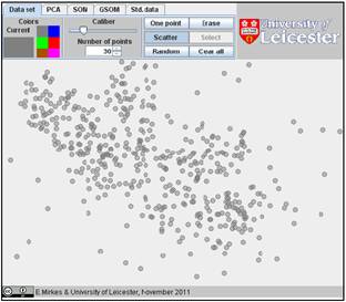
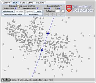
Go
to “PCA” and select by two mouse clicks two points for the initial
approximation of the first principal components.
Click
on the “Learn” button. The four-ray star will be placed at the mean point. This
is not yet a result.
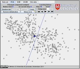
To
watch see the result and the transformation of the straight line from the
initial approximation to the principal component, go to “Learning history”. The
history of iterations will be demonstrated step by step:
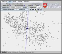

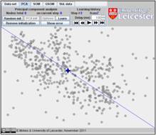
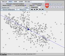
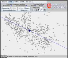

In this example, the iterations converge in seven steps. The result is on the
last figure. The changes at the last three steps are tiny and we have omitted
here the sixth step.
A task for exploration. Usually, the iterations converge in 5-10 steps. Can you find situations
(data sets and initial approximations) when the iterations converge in more
steps? What is the maximum you can achieve in your examples? If you can invent
a data set and initial approximation for which the PCA learning takes 20 or
more steps then you understand the nature of the PCA and learning algorithm.
Please play. You can also organize a competition: who can invent an example
with the maximal number of iterations?
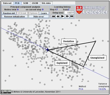
You
can find the accuracy of the approximation of the data set by the first
principal component. For this purpose, use the button “Show error” and find the
value of fraction of variance unexplained (FVU) in
the bottom right corner. This notion is illustrated below. For each data point,
the deviation is the distance from the mean point. The distance from the
projection on the principal component line to the mean point is the explained deviation. The distance from
the data point to the straight line of the first principal component is the unexplained deviation. The ratio of the
sum of squares of these unexplained deviations to the sum of squares of the
deviations from the mean point is the FVU. Usually, it is measured in %.
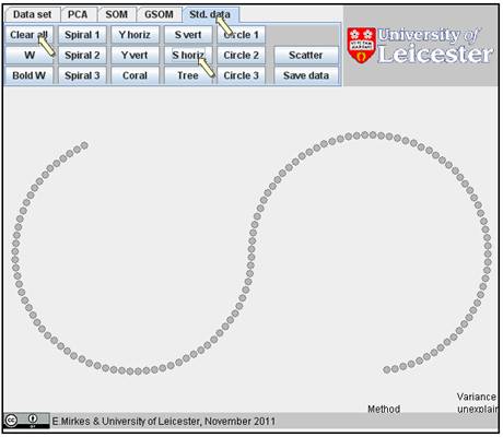
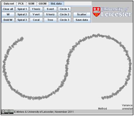
You
can use the standardized data sets: click the button “Std. data”. Clean the
screen and select one of the sets, for example “S horiz.”:
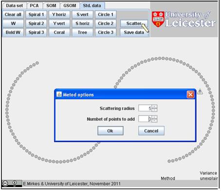
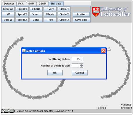
For
smearing of this image, you can use the “Scatter” procedure. Choose the
scattering radius and the number of points to add to every point in a circle
with this radius:
:
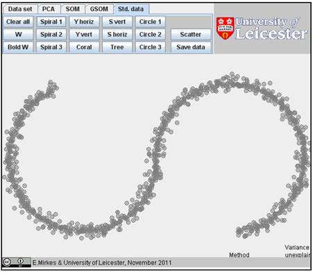
After
you click “OK”, the smeared image appears:
It
may be interesting to use this operation several times with different radii and
numbers of points and prepare a sort of “halo” around the image:
If you add randomly one point to each existent data point in a circle of radius
15, you get the following figure:
Initiate
PCA with two mouse clicks, and learn:
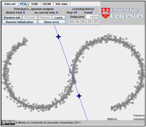
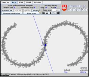
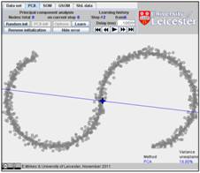
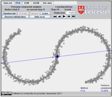
In
our example, the PCA algorithm converges in 6 steps. Go to the Learning history
and look on this history, step by step. Below are the first, second and sixth
steps. The fraction of variance unexplained (FUV) is 18.80%:

Play
with the smeared standard images and explore the possibility of the PCA
approximation. You can also use the Data set/Random button to add noise
uniformly distributed on the work desk
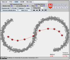
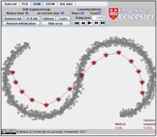
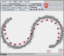
Just
for comparison, below are the self organizing map (SOM) approximations of the
same dataset with 10 nodes (FVU=13.71%), with 15 nodes (FVU=5.50%) and with 20
nodes (FVU=2.62%):
Go
to “First Play With SOM and GSOM” tutorial