The training phase of the algorithm consists only of storing the feature vectors and class labels of the training samples.
In the classification phase, k is a user-defined constant, and an unlabelled vector (a query or test point) is classified by assigning the label which is most frequent among the k training samples nearest to that query point.
Usually Euclidean distance is used as the distance metric; however this is only applicable to continuous variables. In cases such as text classification, another metric such as the overlap metric (or Hamming distance) can be used. Often, the classification accuracy of kNN can be improved significantly if the distance metric is learned with specialized algorithms such as Large Margin Nearest Neighbor or Neighbourhood components analysis.
A drawback to the basic "majority voting" classification is that the classes with the more frequent examples tend to dominate the prediction of the new vector, as they tend to come up in the k nearest neighbors when the neighbors are computed due to their large number. One way to overcome this problem is to weight the classification taking into account the distance from the test point to each of its k nearest neighbors.
KNN can be considered as a special case of a variable-bandwidth, kernel density "balloon" estimator with a uniform kernel.
Some of the labeled training examples may be surround by the examples from the other classes. Such a situation may arise by plenty of reasons: (i) as a resut of a random mistake, (ii) because insufficient number of traning example of this class (an isolated example appears instead of cluster), (iii) because incomplete system of features (the classes are separated in other dimensions which we do not know), (iv) because there are too many training examples of other classes (unbalanced classes) that create too dense "hostile" background for the given small class and many other reasons.
If a training example is surrounded by the examples from other classes it is called the class-outlier. The simplest approach to handle these class-outliers is to detect them and separate for the future analysis. In any case, for the kNN-based classificators they will produce just noise.
KNN approach allows us to detect the class-outliers. Let us select two natural numbers, q≥r>0 . We call a labeled training example the (q,r)NN class-outlier if among its q nearest neighbors there are more than r examples from other classes. In this applet, we always use q=r and consider an example as a qNN class outlier if it has q nearest neighbors from other classes.
Condensend Nearest Neighbor rule (CNN) was invented to reduce the databases for kNN classification. It selects from examples the set of prototypes U that allows us to clasify the example with the 1NN rule "almost" as sucsessful as the 1NN with the initial database does.
The CNN rule (the Hart algorithm) works iteratively. Let us order the set X of the traning examples and numerate them: X={x1, x2, ... xn}. Starting with U={x1}, CNN scans all elements of X. We add to U an example x from X if its nearest prototype from U does not match in label with x. If during the scan of X some new prototypes are added to U then we repeat the scan until no more prototypes are added. After that, we use U instead of X in the classification. The examples that were not included in the set of prototypes are called "absorbed" points. A trivial remark: if an example x is included in U as a prototype then we can exclude it from X and do not test in the following scans.
|
|
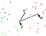
We use an advanced procedure to order the set of all examples X before application of the CNN algorithm. Let x be a labelled example. For them, the external examples are examples with different labels. Let us find a closest to x external example y and then the closest to y example x' with the same label as x. The distance ||x'-y|| never exceed ||x-y||, therefore the ratio a(x)=||x'-y||/||x-y|| belongs to [0,1]. We call it the border ratio. The calculation of the border ration is illustrated by the picture on the left. The data points are labeled by colors. The initial point is x. Its label is red. External points are blue and green. The closest to x external point is y. The closest to y red pont (with the same label as x) is x'. The border ratio a(x)=||x'-y||/||x-y|| is the attribute of the initial point x.
Let us order examples x from X in accordance with the values of a(x), in the descending order (from the biggest to the smallest values with an arbitrary order of the elements with the same values of a) and then apply the CNN procedure. This ordering gives preferencies to the borders of the classes for inclusion in the set of prototypes U.
The applet contains five menu panels (top left), University of Leicester label (top right), work desk (center) and the label of the Attribution 3.0 Creative Commons publication license (bottom).
To wisit the web-site of the University of Leicester click on the University of Leicester logo.
To read the Creative Commons publication license click on the bottom license panel.
|
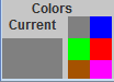
The first part of the Data set panel contains one big coloured rectangle and a pallete built from six small differently coloured rectangles. To select one of the six colors click on a small rectangle. The big coloured rectangle displays the currently selected color..
Different colors are needed to indicate different classes. The points with the same colour are training examples for the same class. To start classification, it is necessary to create the training examples of several classes (several colours).
The third part of the Data set panel contains six buttons. The first three button change the type of cursor brush.
The button "One point" switches the brush to add single points. Every mouse click on the work desk will add a point to the data set.
The button "Scatter" allows you to add several points by one mouse click. You can choose the number of added points in "Number of points" spinner at the middle part of the menu panel. Points are scattered randomly in a circle which radius is determined by the slider "Caliber" in the middle part of menu panel.
The button "Erase" switches the mouse cursore in eraser. When you click the eraser mouse cursor on the work desk, all points, which centres are covered by cursor, are removed from the work desk.
The button "Select" is not used
When you press the "Random" button several points are added on the work desk. The quontity of points is defined by the "Number of points" spinner. The locations of new points are generated randomly on whole work desk.
The button "Erase all" fully clears the work desk. It removes all kinds of object: data points, centroids, test results, maps and so on.
The right hand side of the menu panel "Parameters" gives you the possibility for data reduction. The data reduction here includes two operations: selection of the class-outliers and concentration of data (we implemented here the CNN algorithm with advanced preordering of data according to the border ratio). The class-outliers here are the training examples whose q nearest neighbors belong to the other classes. You can choose this number of NNs for outlier detection. Its default value is q=3.
|
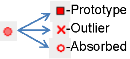
"Implement reduction". When you press this button, each data point transforms into a sample of one of three different types. It can become a prototype (they are displayed as squares). It can be transformed into an outlier (a cross) or an absorbed point (an empty circle). After data reduction, the absorbed data points and the outliers do not participate in the classification tasks, testing and mapping. In the left bottom corner of the work desk the percents of prototypes, outliers and absorbed elements are displayed for each class
Warning. After the CNN procedure the best result in testing and validation gives the 1NN classification algorithm (or the method of protential energy). The kNN method with k>1 does not work properly after this type of data reduction. The cross - validation will demonstrate you that it is almost impossible to delete any prototype from reduced data.
The "Unselect" button cancels the data reduction results and returns the previous picture.